Naive Bayesian Classifier
Prior, posterior probability
이전에 prior probability와 posterior probability에 대해서 공부했다.
다시 요약해 보자면 ...
θ에 관심이 있다고 할 때,
- prior probability: 데이터를 모으거나 측정하기 전의 θ에 대한 uncertainty를 나타낸다.
distribution 표현: π(θ)
- posterior probability: 데이터를 모으거나 측정한 후의 θ에 대한 uncertainty를 나타낸다.
distribution 표현: π(θ|X)
관찰된 데이터에 대한 조건부 확률이다.
위 확률 개념은 Bayes' theorem에 기반을 둔 Naive Bayesian Classifier에서 사용된다.
Naive Bayesian 모델은 복잡한 parameter estimation 반복이 없어 구성하기 쉽고, 특히 매우 큰 데이터셋에 유용하다.
모델이 이렇게 단순해도 좋은 성능을 보여준다.
Bayes theorem
Bayes theorem은 P(c), P(x), P(x|c)로부터 posterior probability인 P(c|x)를 계산하는 방법이다.
Naive Bayes classifier는 predictor (x)의 class (c) 에 대한 값의 효과가 다른 prodictor들의 값과 독립적이라고 가정한다.
이 가정은 class conditional independence - 클래스 조건 독립 이라고 불린다.
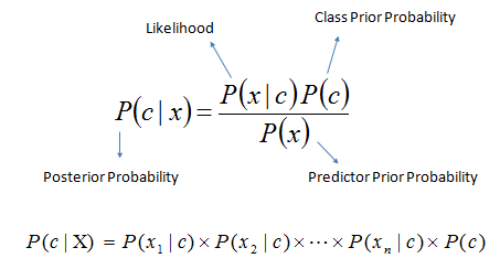
P(c|x): predictor(attribute)가 주어졌을 때 class(target)의 posterior probability.
P(c): the prior probability of class
P(x|c): Likelihood = probability of predictor given class
P(x): the prior probability of predictor
Bayesian deep learning을 통해 uncertainty 보완될 수 있었다.
Naive Bayesian Classifier - 예시

위 사진과 같은 일기예보 데이터셋이 있다. Input feature은 4개이고 (4 dimension) output은 binary이다.
이 데이터셋에서 prediction을 구하기 위해 posterior probability를 계산하는 방법은 다음과 같다.
1. target(class)에 대한 각 attribute(predictor)의 frequency table을 작성한다.
2. frequency table을 likelihood table로 변환한다.
3. Naive Bayesian equation을 사용해서 각 class에 대한 posterior probability를 계산한다.
4. 가장 높은 posterior probability를 가진 class가 prediction의 결과이다.
